Compressing a 1D CNN for Edge AI: Results, Limits and Trade-offs
How much classification quality can we keep when model size and latency become important limits for deployment?
This article studies a simple human activity recognition task based on inertial signals. The goal is not to find one compression method that is always better. Instead, the goal is to measure the effects of three decisions:
- Reduce the model capacity with a Student architecture
- Train this Student with knowledge distillation
- Quantize the model after training with PTQ or during fine-tuning with QAT
This difference is important. Most of the reduction in the number of parameters comes from the Student architecture. Distillation improves how the Student learns without changing its size. Quantization changes the numerical format of the weights and some activations.
Dataset and classification task
This study uses the UCI Human Activity Recognition Using Smartphones dataset. It contains measurements from 30 people who wore a smartphone on their waist. The sensors recorded data at 50 Hz. The signals were then divided into windows of 128 samples, which represent 2.56 seconds, with an overlap of 50%.
The dataset provides several inertial signals. This project uses six channels: the three axes of estimated body acceleration and the three axes of angular velocity. Each window belongs to one of six activities:
- Walking
- Walking upstairs
- Walking downstairs
- Sitting
- Standing
- Lying down

Why use a 1D CNN for an IMU signal?
An IMU window is a short time series with several channels. The input tensor uses
the (batch, channels, time) order. In this project, its shape is (B, 6, 128).
A 1D convolution can learn local patterns over time, such as the rhythm of
walking, a change of movement, the impact of a step, or a link between
acceleration and rotation.
A convolutional filter uses the same weights across the whole time window. It can therefore detect the same pattern, such as the impact of a step, at any position in the window without learning different weights for each time step. Unlike a recurrent network, a CNN can process several positions in parallel. Finally, the small number of layers and filters makes it possible to build a compact Student model with 5,462 parameters.
An LSTM could be useful if the model needed to learn relationships longer than the current window. A Transformer could be useful for longer sequences or when long-range relationships justify the cost of attention. A 1D CNN is not the best choice for every task. Here, it is suitable because the windows are short, the sampling rate is fixed, and the target CPU has limited resources.
Experimental method
The official test set contains 2,947 windows. The training set is divided into training and validation groups by person. The same person cannot appear in both groups. This prevents data leakage between strongly related windows, especially because two following windows overlap by 50%.
The normalization values used for validation and testing are calculated only from the training group. The same values are then used in the Python and C++ pipelines.
The inference benchmark uses:
- A fixed input with shape
(1, 6, 128) - 100 warm-up inferences
- 2,000 measured inferences
- A new process for each model
ORT_SEQUENTIALwith one intra-op threadORT_ENABLE_ALLin both implementations- No model loading time in the measurements
- Separate results for the mean and the p50, p95 and p99 values
The measurements were made on Windows with an AMD Ryzen 5 5600 processor
(6 cores and 12 threads), Python 3.11, and the ONNX Runtime
CPUExecutionProvider. The exact software versions should be taken from the
environment that produced the results. This includes the output of pip freeze
and the version of the C++ library. These details are needed to reproduce the
benchmark.
This method measures stable inference latency after the warm-up phase on one logical core. It does not include the first cold run, IMU data collection, window creation, or normalization. Reusing an input with the same size also reduces variation and helps the CPU caches. For these reasons, the results do not show the full end-to-end latency of an embedded system.
Three groups of compression methods
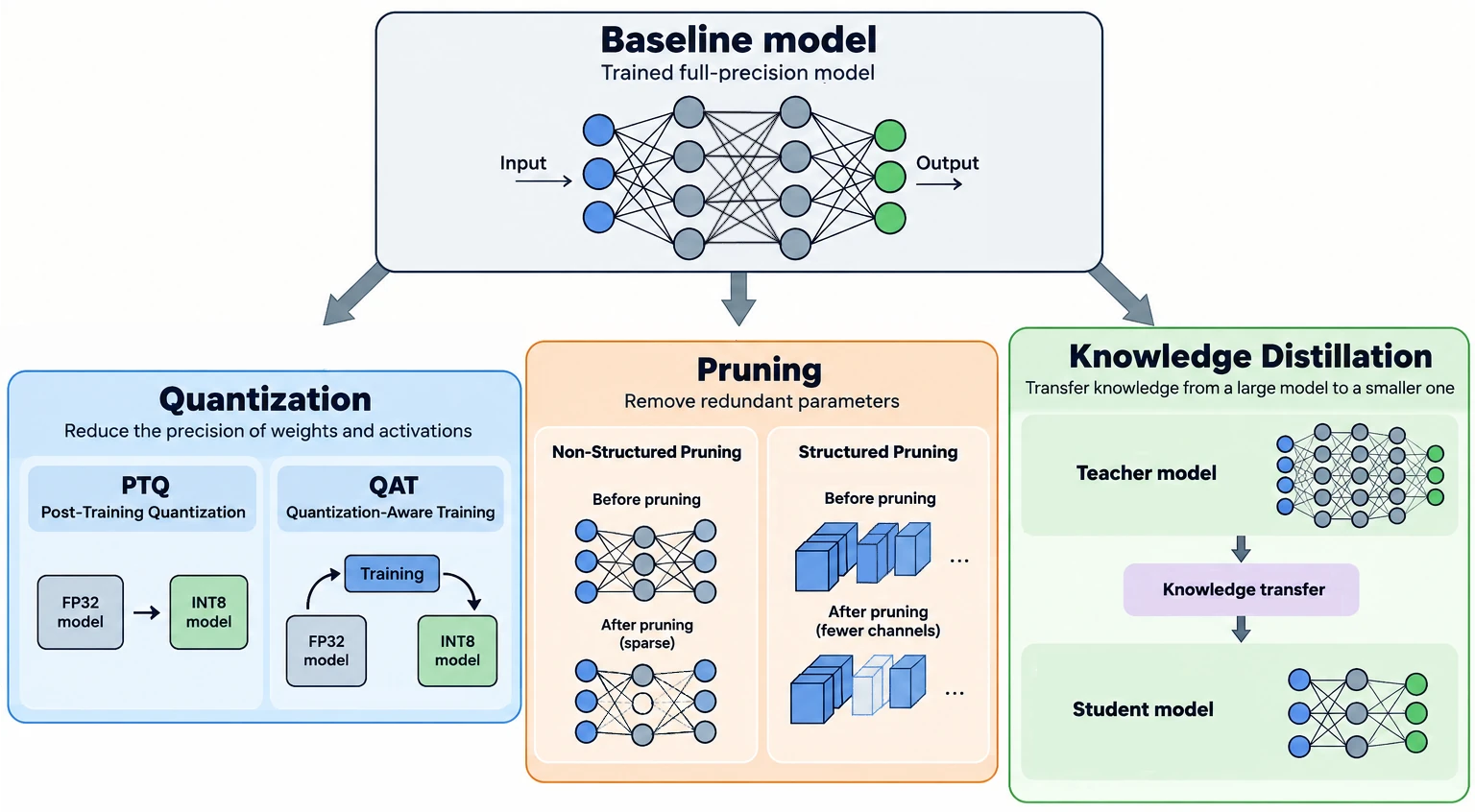 Overview of quantization, pruning and knowledge distillation
The figure shows three common groups of methods. This article measures distillation and quantization. Pruning is included to give a wider view of model compression, but it is not part of the results.
- Unstructured pruning sets individual weights to zero. This creates many zero values, but it does not automatically reduce latency or file size. It needs a sparse storage format and suitable compute kernels
- Structured pruning removes complete parts of the network, such as channels or filters. It can directly change the network dimensions. It is usually easier to use on general hardware, but it may cause a larger quality loss for the same pruning rate
Distillation: learning more than one label
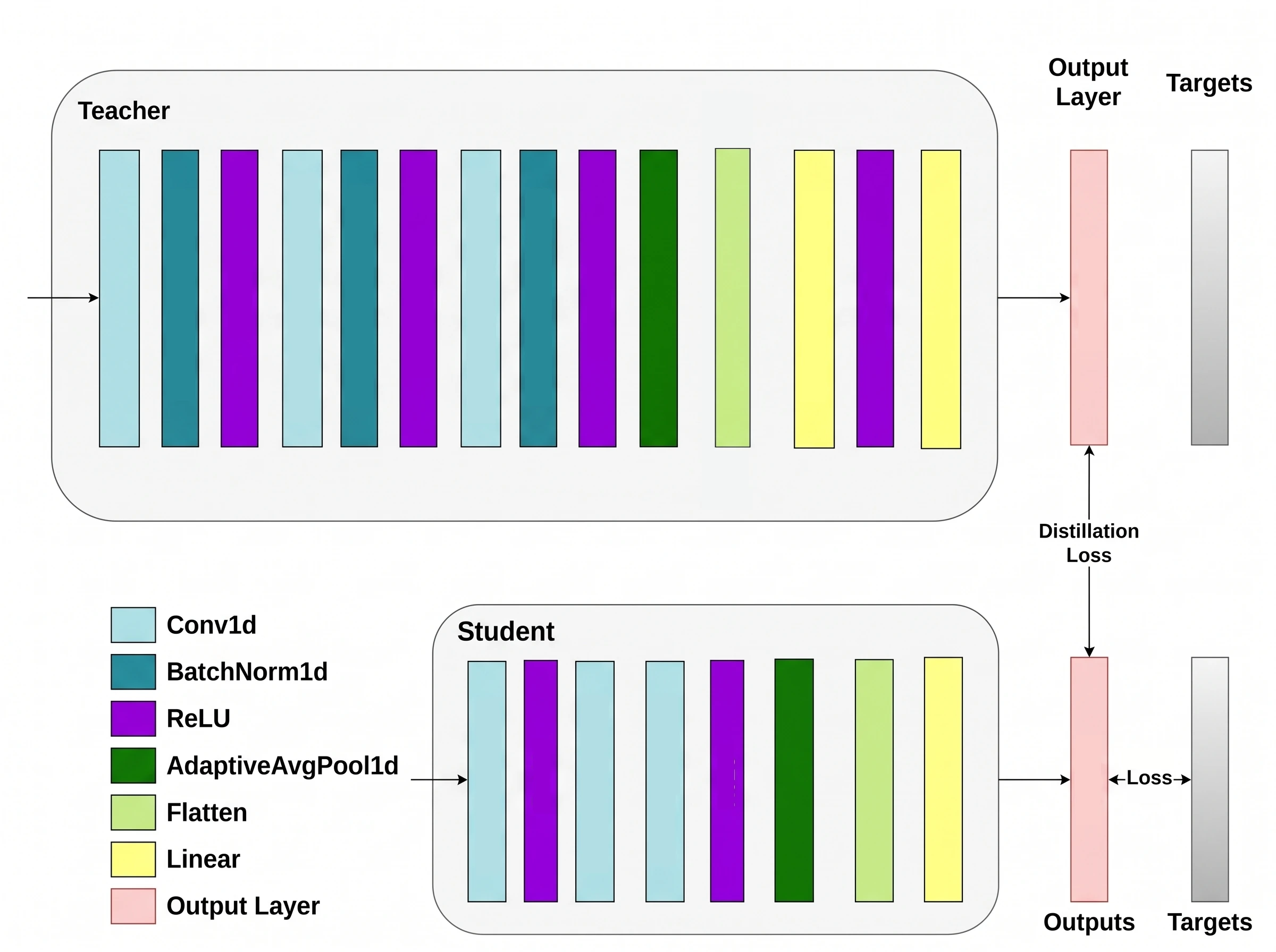 Teacher and Student architectures
The baseline Student learns with a standard cross-entropy loss. For a walking
window, the target only shows that WALKING is the correct class. It does not
show that WALKING_UPSTAIRS is a more likely mistake than LAYING.
Knowledge distillation adds the Teacher output distribution as another training signal. The loss function is:
Here, and are the Teacher and Student logits, is the temperature, and controls the importance of distillation. The factor corrects the change in gradient scale caused by the temperature.
The Student architecture and its 5,462 parameters stay unchanged. Distillation does not directly compress this network. It helps an already small model use its capacity more effectively. The Teacher is only needed during training.
Post-Training Quantization (PTQ)
In this study, Post-Training Quantization is applied after training. A group of
1,024 representative windows from the training set is used to calibrate the
activation ranges. The weights are quantized per channel, and the ONNX model uses
the QDQ format with QuantizeLinear and DequantizeLinear operators.
If the calibration range is too small, extreme values are clipped. If the range is too large, each quantization step becomes larger and small changes are harder to represent. For this reason, the calibration data should cover the different people, activities, signal levels, peaks, and noise levels expected during real use.
PTQ does not need any new training. However, a QDQ graph does not mean that every operator runs with 8-bit integers. This depends on the operators, the available compute kernels, and the Execution Provider. Inputs and outputs may also stay in FP32 around quantized parts of the graph.
Quantization-Aware Training (QAT)
QAT starts from the distilled Student and simulates quantization during fine-tuning. In this setup, the activations use simulated UINT8 quantization. The weights of the convolution and linear layers use simulated INT8 quantization with one scale for each output channel.
During the forward pass, fake quantization simulates rounding, clipping, and dequantization while keeping floating-point tensors for training. Backpropagation then allows the weights to adapt to these numerical errors. QAT needs an extra training stage, but it often keeps more quality when PTQ does not meet the target error limit.
Training and deployment pipeline
Results
The FP32 Teacher reaches an F1-score of 0.90 with 176,966 parameters. The baseline Student has only 5,462 parameters and reaches 0.69. It has 32.4 times fewer parameters, but this smaller architecture is also the main cause of the quality loss.
Distillation raises the F1-score of the same Student to 0.76 without changing its architecture. PTQ reaches 0.72. QAT reaches 0.75. In this experiment, QAT keeps almost all the F1-score of the distilled Student while producing the smallest file.
Summary table
| Model | Format | Parameters | ONNX size | p95 Python / C++ | F1-score |
|---|---|---|---|---|---|
| Teacher 1D CNN | FP32 | 176,966 | 689.9 KiB | 514.6 / 528.0 µs | 0.90 |
| Baseline Student | FP32 | 5,462 | 23.1 KiB | 82.5 / 42.2 µs | 0.69 |
| Distilled Student | FP32 | 5,462 | 23.1 KiB | 65.0 / 50.2 µs | 0.76 |
| Distilled Student PTQ | QDQ, U8/S8 | 5,462 | 15.3 KiB | 64.0 / 42.8 µs | 0.72 |
| Distilled Student QAT | QDQ, U8/S8 | 5,462 | 10.9 KiB | 63.4 / 45.7 µs | 0.75 |
The QAT file is about 63 times smaller than the Teacher file. However, this comparison includes two changes: the new Student architecture and quantization. To measure only the effect of quantization, QAT should be compared with the distilled FP32 Student. The file size then falls from 23.1 KiB to 10.9 KiB, which is a reduction of about 2.1 times.
Quality and latency trade-off
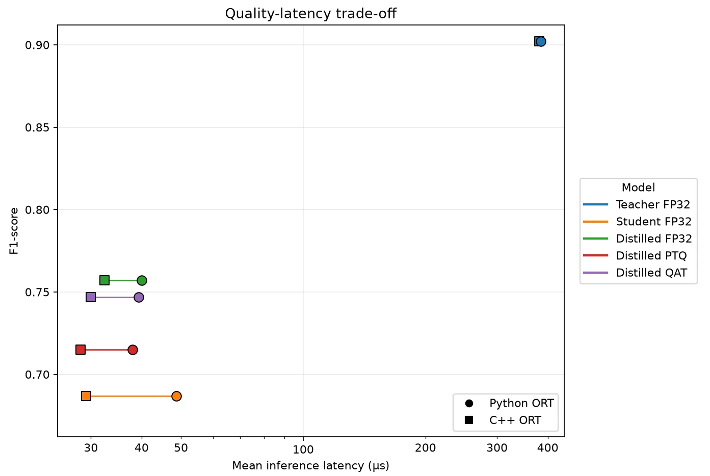 F1-score compared with average latency
The Teacher is in a separate area of the graph. Its F1-score is clearly higher, but its latency is also longer. Among the small models, the distilled FP32 Student keeps the best F1-score. QAT has a slightly lower score, but it produces the smallest file. The coloured lines connect the Python and C++ measurements of the same ONNX file. Circles show Python results, and squares show C++ results.
Quantization does not automatically make this small network faster on the Ryzen 5 5600. Q/DQ conversions, available compute kernels, fixed runtime costs, and the very small amount of computation can hide the benefit of INT8. In this test, most of the latency improvement comes from replacing the Teacher with the Student.
Limits of the study
This experiment uses one random seed, one validation split, and one computer. It does not provide a confidence interval, a distribution across several training runs, or an energy measurement.
The benchmark only measures ONNX Runtime with an input that is already prepared. A complete Edge AI deployment should also measure:
- Data collection, window creation, and normalization
- Peak RAM use, not only the file size (RSS)
- Start-up time and the first inference
- Latency under load and energy use
- The confusion matrix, especially for
SITTINGandSTANDING - Performance with new people, sensor positions, and noise levels
A more complete study would repeat training with several random seeds, use several data splits based on people, and report the mean, standard deviation, or confidence interval.
Conclusion
The results lead to four main observations:
- The Student architecture has 32.4 times fewer parameters than the Teacher, but it loses an important part of the model quality
- Distillation recovers 7.0 F1-score points without adding parameters
- PTQ is easy to apply, but it reduces the quality of the distilled Student in this experiment
- QAT keeps 98.7% of the distilled Student F1-score and reduces its file size by about 2.1 times
The distilled FP32 Student is still the best choice among the small models when the F1-score is the main goal. QAT is a better choice when storage is more limited and a decrease of 0.01 in the F1-score is acceptable. On a real embedded target, the final choice must be tested again with its compute kernels, memory limits, and energy budget. An x86 benchmark cannot fully predict the behaviour of a microcontroller or an AI accelerator.